Understanding PLONK
2019 Sep 22
See all posts
Understanding PLONK
Special thanks to Justin Drake, Karl Floersch, Hsiao-wei Wang,
Barry Whitehat, Dankrad Feist, Kobi Gurkan and Zac Williamson for
review
Very recently, Ariel Gabizon, Zac Williamson and Oana Ciobotaru
announced a new general-purpose zero-knowledge proof scheme called PLONK, standing for the
unwieldy quasi-backronym "Permutations over Lagrange-bases for
Oecumenical Noninteractive arguments of Knowledge". While improvements to
general-purpose zero-knowledge proof
protocols have been coming
for years, what PLONK
(and the earlier but more complex SONIC
and the more recent Marlin) bring to the
table is a series of enhancements that may greatly improve the usability
and progress of these kinds of proofs in general.
The first improvement is that while PLONK still requires a trusted
setup procedure similar to that needed for the SNARKs in Zcash,
it is a "universal and updateable" trusted setup. This means two things:
first, instead of there being one separate trusted setup for every
program you want to prove things about, there is one single trusted
setup for the whole scheme after which you can use the scheme with any
program (up to some maximum size chosen when making the setup). Second,
there is a way for multiple parties to participate in the trusted setup
such that it is secure as long as any one of them is honest, and this
multi-party procedure is fully sequential: first one person
participates, then the second, then the third... The full set of
participants does not even need to be known ahead of time; new
participants could just add themselves to the end. This makes it easy
for the trusted setup to have a large number of participants, making it
quite safe in practice.
The second improvement is that the "fancy cryptography" it relies on
is one single standardized component, called a "polynomial commitment".
PLONK uses "Kate commitments", based on a trusted setup and elliptic
curve pairings, but you can instead swap it out with other schemes, such
as FRI (which would
turn PLONK into a kind of
STARK) or DARK (based on hidden-order groups). This means the scheme
is theoretically compatible with any (achievable) tradeoff between proof
size and security assumptions.
What this means is that use cases that require different tradeoffs
between proof size and security assumptions (or developers that have
different ideological positions about this question) can still share the
bulk of the same tooling for "arithmetization" - the process for
converting a program into a set of polynomial equations that the
polynomial commitments are then used to check. If this kind of scheme
becomes widely adopted, we can thus expect rapid progress in improving
shared arithmetization techniques.
How PLONK works
Let us start with an explanation of how PLONK works, in a somewhat
abstracted format that focuses on polynomial equations without
immediately explaining how those equations are verified. A key
ingredient in PLONK, as is the case in the QAPs
used in SNARKs, is a procedure for converting a problem of the form
"give me a value \(X\) such that a
specific program \(P\) that I give you,
when evaluated with \(X\) as an input,
gives some specific result \(Y\)" into
the problem "give me a set of values that satisfies a set of math
equations". The program \(P\) can
represent many things; for example the problem could be "give me a
solution to this sudoku", which you would encode by setting \(P\) to be a sudoku verifier plus some
initial values encoded and setting \(Y\) to \(1\) (ie. "yes, this solution is correct"),
and a satisfying input \(X\) would be a
valid solution to the sudoku. This is done by representing \(P\) as a circuit with logic gates for
addition and multiplication, and converting it into a system of
equations where the variables are the values on all the wires and there
is one equation per gate (eg. \(x_6 = x_4
\cdot x_7\) for multiplication, \(x_8 =
x_5 + x_9\) for addition).
Here is an example of the problem of finding \(x\) such that \(P(x) = x^3 + x + 5 = 35\) (hint: \(x = 3\)):
We can label the gates and wires as follows:
On the gates and wires, we have two types of constraints:
gate constraints (equations between wires attached to
the same gate, eg. \(a_1 \cdot b_1 =
c_1\)) and copy constraints (claims about
equality of different wires anywhere in the circuit, eg. \(a_0 = a_1 = b_1 = b_2 = a_3\) or \(c_0 = a_1\)). We will need to create a
structured system of equations, which will ultimately reduce to a very
small number of polynomial equations, to represent both.
In PLONK, the setup for these equations is as follows. Each equation
is of the following form (think: \(L\)
= left, \(R\) = right, \(O\) = output, \(M\) = multiplication, \(C\) = constant):
\[
\left(Q_{L_{i}}\right) a_{i}+\left(Q_{R_{i}}\right)
b_{i}+\left(Q_{O_{i}}\right) c_{i}+\left(Q_{M_{i}}\right) a_{i}
b_{i}+Q_{C_{i}}=0
\]
Each \(Q\) value is a constant; the
constants in each equation (and the number of equations) will be
different for each program. Each small-letter value is a variable,
provided by the user: \(a_i\) is the
left input wire of the \(i\)'th gate,
\(b_i\) is the right input wire, and
\(c_i\) is the output wire of the \(i\)'th gate. For an addition gate, we
set:
\[
Q_{L_{i}}=1, Q_{R_{i}}=1, Q_{M_{i}}=0, Q_{O_{i}}=-1, Q_{C_{i}}=0
\]
Plugging these constants into the equation and simplifying gives us
\(a_i + b_i - c_i = 0\), which is
exactly the constraint that we want. For a multiplication gate, we
set:
\[
Q_{L_{i}}=0, Q_{R_{i}}=0, Q_{M_{i}}=1, Q_{O_{i}}=-1, Q_{C_{i}}=0
\]
For a constant gate setting \(a_i\)
to some constant \(x\), we set:
\[
Q_{L}=1, Q_{R}=0, Q_{M}=0, Q_{O}=0, Q_{C}=-x
\]
You may have noticed that each end of a wire, as well as each wire in
a set of wires that clearly must have the same value (eg. \(x\)), corresponds to a distinct variable;
there's nothing so far forcing the output of one gate to be the same as
the input of another gate (what we call "copy constraints"). PLONK does
of course have a way of enforcing copy constraints, but we'll get to
this later. So now we have a problem where a prover wants to prove that
they have a bunch of \(x_{a_i},
x_{b_i}\) and \(x_{c_i}\) values
that satisfy a bunch of equations that are of the same form. This is
still a big problem, but unlike "find a satisfying input to this
computer program" it's a very structured big problem, and we
have mathematical tools to "compress" it.
From linear systems to
polynomials
If you have read about STARKs or QAPs,
the mechanism described in this next section will hopefully feel
somewhat familiar, but if you have not that's okay too. The main
ingredient here is to understand a polynomial as a mathematical
tool for encapsulating a whole lot of values into a single object.
Typically, we think of polynomials in "coefficient form", that is an
expression like:
\[
y=x^{3}-5 x^{2}+7 x-2
\]
But we can also view polynomials in "evaluation form". For example,
we can think of the above as being "the" degree \(< 4\) polynomial with evaluations \((-2, 1, 0, 1)\) at the coordinates \((0, 1, 2, 3)\) respectively.
Now here's the next step. Systems of many equations of the same form
can be re-interpreted as a single equation over polynomials. For
example, suppose that we have the system:
\[
\begin{array}{l}{2 x_{1}-x_{2}+3 x_{3}=8} \\ {x_{1}+4 x_{2}-5 x_{3}=5}
\\ {8 x_{1}-x_{2}-x_{3}=-2}\end{array}
\]
Let us define four polynomials in evaluation form: \(L(x)\) is the degree \(< 3\) polynomial that evaluates to \((2, 1, 8)\) at the coordinates \((0, 1, 2)\), and at those same coordinates
\(M(x)\) evaluates to \((-1, 4, -1)\), \(R(x)\) to \((3,
-5, -1)\) and \(O(x)\) to \((8, 5, -2)\) (it is okay to directly define
polynomials in this way; you can use Lagrange
interpolation to convert to coefficient form). Now, consider the
equation:
\[
L(x) \cdot x_{1}+M(x) \cdot x_{2}+R(x) \cdot x_{3}-O(x)=Z(x) H(x)
\]
Here, \(Z(x)\) is shorthand for
\((x-0) \cdot (x-1) \cdot (x-2)\) - the
minimal (nontrivial) polynomial that returns zero over the evaluation
domain \((0, 1, 2)\). A solution to
this equation (\(x_1 = 1, x_2 = 6, x_3 = 4,
H(x) = 0\)) is also a solution to the original system of
equations, except the original system does not need \(H(x)\). Notice also that in this case,
\(H(x)\) is conveniently zero, but in
more complex cases \(H\) may need to be
nonzero.
So now we know that we can represent a large set of constraints
within a small number of mathematical objects (the polynomials). But in
the equations that we made above to represent the gate wire constraints,
the \(x_1, x_2, x_3\) variables are
different per equation. We can handle this by making the variables
themselves polynomials rather than constants in the same way. And so we
get:
\[
Q_{L}(x) a(x)+Q_{R}(x) b(x)+Q_{O}(x) c(x)+Q_{M}(x) a(x) b(x)+Q_{C}(x)=0
\]
As before, each \(Q\) polynomial is
a parameter that can be generated from the program that is being
verified, and the \(a\), \(b\), \(c\)
polynomials are the user-provided inputs.
Copy constraints
Now, let us get back to "connecting" the wires. So far, all we have
is a bunch of disjoint equations about disjoint values that are
independently easy to satisfy: constant gates can be satisfied by
setting the value to the constant and addition and multiplication gates
can simply be satisfied by setting all wires to zero! To make the
problem actually challenging (and actually represent the problem encoded
in the original circuit), we need to add an equation that verifies "copy
constraints": constraints such as \(a(5) =
c(7)\), \(c(10) = c(12)\), etc.
This requires some clever trickery.
Our strategy will be to design a "coordinate pair accumulator", a
polynomial \(p(x)\) which works as
follows. First, let \(X(x)\) and \(Y(x)\) be two polynomials representing the
\(x\) and \(y\) coordinates of a set of points (eg. to
represent the set \(((0, -2), (1, 1), (2, 0),
(3, 1))\) you might set \(X(x) =
x\) and \(Y(x) = x^3 - 5x^2 + 7x -
2)\). Our goal will be to let \(p(x)\) represent all the points up to (but
not including) the given position, so \(p(0)\) starts at \(1\), \(p(1)\) represents just the first point,
\(p(2)\) the first and the second, etc.
We will do this by "randomly" selecting two constants, \(v_1\) and \(v_2\), and constructing \(p(x)\) using the constraints \(p(0) = 1\) and \(p(x+1) = p(x) \cdot (v_1 + X(x) + v_2 \cdot
Y(x))\) at least within the domain \((0, 1, 2, 3)\).
For example, letting \(v_1 = 3\) and
\(v_2 = 2\), we get:
|
X(x)
|
0
|
1
|
2
|
3
|
4
|
|
\(Y(x)\)
|
-2
|
1
|
0
|
1
|
|
|
\(v_1 + X(x) + v_2 \cdot
Y(x)\)
|
-1
|
6
|
5
|
8
|
|
|
\(p(x)\)
|
1
|
-1
|
-6
|
-30
|
-240
|
Notice that (aside from the first column) every \(p(x)\) value equals the value to the left
of it multiplied by the value to the left and above it.
The result we care about is \(p(4) =
-240\). Now, consider the case where instead of \(X(x) = x\), we set \(X(x) = \frac{2}{3} x^3 - 4x^2 +
\frac{19}{3}x\) (that is, the polynomial that evaluates to \((0, 3, 2, 1)\) at the coordinates \((0, 1, 2, 3)\)). If you run the same
procedure, you'll find that you also get \(p(4) = -240\). This is not a coincidence
(in fact, if you randomly pick \(v_1\)
and \(v_2\) from a sufficiently large
field, it will almost never happen coincidentally). Rather,
this happens because \(Y(1) = Y(3)\),
so if you "swap the \(X\) coordinates"
of the points \((1, 1)\) and \((3, 1)\) you're not changing the
set of points, and because the accumulator encodes a set (as
multiplication does not care about order) the value at the end will be
the same.
Now we can start to see the basic technique that we will use to prove
copy constraints. First, consider the simple case where we only want to
prove copy constraints within one set of wires (eg. we want to prove
\(a(1) = a(3)\)). We'll make two
coordinate accumulators: one where \(X(x) =
x\) and \(Y(x) = a(x)\), and the
other where \(Y(x) = a(x)\) but \(X'(x)\) is the polynomial that
evaluates to the permutation that flips (or otherwise rearranges) the
values in each copy constraint; in the \(a(1)
= a(3)\) case this would mean the permutation would start \(0 3 2 1 4...\). The first accumulator would
be compressing \(((0, a(0)), (1, a(1)), (2,
a(2)), (3, a(3)), (4, a(4))...\), the second \(((0, a(0)), (3, a(1)), (2, a(2)), (1, a(3)), (4,
a(4))...\). The only way the two can give the same result is if
\(a(1) = a(3)\).
To prove constraints between \(a\),
\(b\) and \(c\), we use the same procedure, but instead
"accumulate" together points from all three polynomials. We assign each
of \(a\), \(b\), \(c\)
a range of \(X\) coordinates (eg. \(a\) gets \(X_a(x)
= x\) ie. \(0...n-1\), \(b\) gets \(X_b(x)
= n+x\), ie. \(n...2n-1\), \(c\) gets \(X_c(x)
= 2n+x\), ie. \(2n...3n-1\). To
prove copy constraints that hop between different sets of wires, the
"alternate" \(X\) coordinates would be
slices of a permutation across all three sets. For example, if we want
to prove \(a(2) = b(4)\) with \(n = 5\), then \(X'_a(x)\) would have evaluations \(\{0, 1, 9, 3, 4\}\) and \(X'_b(x)\) would have evaluations \(\{5, 6, 7, 8, 2\}\) (notice the \(2\) and \(9\) flipped, where \(9\) corresponds to the \(b_4\) wire). Often, \(X'_a(x)\), \(X'_b(x)\) and \(X'_c(x)\) are also called \(\sigma_a(x)\), \(\sigma_b(x)\) and \(\sigma_c(x)\).
We would then instead of checking equality within one run of the
procedure (ie. checking \(p(4) =
p'(4)\) as before), we would check the product of
the three different runs on each side:
\[
p_{a}(n) \cdot p_{b}(n) \cdot p_{c}(n)=p_{a}^{\prime}(n) \cdot
p_{b}^{\prime}(n) \cdot p_{c}^{\prime}(n)
\]
The product of the three \(p(n)\)
evaluations on each side accumulates all coordinate pairs in
the \(a\), \(b\) and \(c\) runs on each side together, so this
allows us to do the same check as before, except that we can now check
copy constraints not just between positions within one of the three sets
of wires \(a\), \(b\) or \(c\), but also between one set of wires and
another (eg. as in \(a(2) =
b(4)\)).
And that's all there is to it!
Putting it all together
In reality, all of this math is done not over integers, but over a
prime field; check the section "A Modular Math Interlude" here for a description
of what prime fields are. Also, for mathematical reasons perhaps best
appreciated by reading and understanding this article on FFT
implementation, instead of representing wire indices with \(x=0....n-1\), we'll use powers of \(\omega: 1, \omega, \omega ^2....\omega
^{n-1}\) where \(\omega\) is a
high-order root-of-unity in the field. This changes nothing about the
math, except that the coordinate pair accumulator constraint checking
equation changes from \(p(x + 1) = p(x) \cdot
(v_1 + X(x) + v_2 \cdot Y(x))\) to \(p(\omega \cdot x) = p(x) \cdot (v_1 + X(x) + v_2
\cdot Y(x))\), and instead of using \(0..n-1\), \(n..2n-1\), \(2n..3n-1\) as coordinates we use \(\omega^i, g \cdot \omega^i\) and \(g^2 \cdot \omega^i\) where \(g\) can be some random high-order element
in the field.
Now let's write out all the equations we need to check. First, the
main gate-constraint satisfaction check:
\[
Q_{L}(x) a(x)+Q_{R}(x) b(x)+Q_{O}(x) c(x)+Q_{M}(x) a(x) b(x)+Q_{C}(x)=0
\]
Then the polynomial accumulator transition constraint (note: think of
"\(= Z(x) \cdot H(x)\)" as meaning
"equals zero for all coordinates within some particular domain that we
care about, but not necessarily outside of it"):
\[
\begin{array}{l}{P_{a}(\omega x)-P_{a}(x)\left(v_{1}+x+v_{2} a(x)\right)
=Z(x) H_{1}(x)} \\ {P_{a^{\prime}}(\omega
x)-P_{a^{\prime}}(x)\left(v_{1}+\sigma_{a}(x)+v_{2} a(x)\right)=Z(x)
H_{2}(x)} \\ {P_{b}(\omega x)-P_{b}(x)\left(v_{1}+g x+v_{2}
b(x)\right)=Z(x) H_{3}(x)} \\ {P_{b^{\prime}}(\omega
x)-P_{b^{\prime}}(x)\left(v_{1}+\sigma_{b}(x)+v_{2} b(x)\right)=Z(x)
H_{4}(x)} \\ {P_{c}(\omega x)-P_{c}(x)\left(v_{1}+g^{2} x+v_{2}
c(x)\right)=Z(x) H_{5}(x)} \\ {P_{c^{\prime}}(\omega
x)-P_{c^{\prime}}(x)\left(v_{1}+\sigma_{c}(x)+v_{2} c(x)\right)=Z(x)
H_{6}(x)}\end{array}
\]
Then the polynomial accumulator starting and ending constraints:
\[
\begin{array}{l}{P_{a}(1)=P_{b}(1)=P_{c}(1)=P_{a^{\prime}}(1)=P_{b^{\prime}}(1)=P_{c^{\prime}}(1)=1}
\\ {P_{a}\left(\omega^{n}\right) P_{b}\left(\omega^{n}\right)
P_{c}\left(\omega^{n}\right)=P_{a^{\prime}}\left(\omega^{n}\right)
P_{b^{\prime}}\left(\omega^{n}\right)
P_{c^{\prime}}\left(\omega^{n}\right)}\end{array}
\]
The user-provided polynomials are:
- The wire assignments \(a(x), b(x),
c(x)\)
- The coordinate accumulators \(P_a(x),
P_b(x), P_c(x), P_{a'}(x), P_{b'}(x),
P_{c'}(x)\)
- The quotients \(H(x)\) and \(H_1(x)...H_6(x)\)
The program-specific polynomials that the prover and verifier need to
compute ahead of time are:
- \(Q_L(x), Q_R(x), Q_O(x), Q_M(x),
Q_C(x)\), which together represent the gates in the circuit (note
that \(Q_C(x)\) encodes public inputs,
so it may need to be computed or modified at runtime)
- The "permutation polynomials" \(\sigma_a(x), \sigma_b(x)\) and \(\sigma_c(x)\), which encode the copy
constraints between the \(a\), \(b\) and \(c\) wires
Note that the verifier need only store commitments to these
polynomials. The only remaining polynomial in the above equations is
\(Z(x) = (x - 1) \cdot (x - \omega) \cdot ...
\cdot (x - \omega ^{n-1})\) which is designed to evaluate to zero
at all those points. Fortunately, \(\omega\) can be chosen to make this
polynomial very easy to evaluate: the usual technique is to choose \(\omega\) to satisfy \(\omega ^n = 1\), in which case \(Z(x) = x^n - 1\).
There is one nuance here: the constraint between \(P_a(\omega^{i+1})\) and \(P_a(\omega^i)\) can't be true across the
entire circle of powers of \(\omega\); it's almost always false at \(\omega^{n-1}\) as the next coordinate is
\(\omega^n = 1\) which brings us back
to the start of the "accumulator"; to fix this, we can modify
the constraint to say "either the constraint is true
or \(x = \omega^{n-1}\)",
which one can do by multiplying \(x -
\omega^{n-1}\) into the constraint so it equals zero at that
point.
The only constraint on \(v_1\) and
\(v_2\) is that the user must not be
able to choose \(a(x), b(x)\) or \(c(x)\) after \(v_1\) and \(v_2\) become known, so we can satisfy this
by computing \(v_1\) and \(v_2\) from hashes of commitments to \(a(x), b(x)\) and \(c(x)\).
So now we've turned the program satisfaction problem into a simple
problem of satisfying a few equations with polynomials, and there are
some optimizations in PLONK that allow us to remove many of the
polynomials in the above equations that I will not go into to preserve
simplicity. But the polynomials themselves, both the program-specific
parameters and the user inputs, are big. So the next
question is, how do we get around this so we can make the proof
short?
Polynomial commitments
A polynomial
commitment is a short object that "represents" a polynomial, and
allows you to verify evaluations of that polynomial, without needing to
actually contain all of the data in the polynomial. That is, if someone
gives you a commitment \(c\)
representing \(P(x)\), they can give
you a proof that can convince you, for some specific \(z\), what the value of \(P(z)\) is. There is a further mathematical
result that says that, over a sufficiently big field, if certain kinds
of equations (chosen before \(z\) is
known) about polynomials evaluated at a random \(z\) are true, those same equations are true
about the whole polynomial as well. For example, if \(P(z) \cdot Q(z) + R(z) = S(z) + 5\), then
we know that it's overwhelmingly likely that \(P(x) \cdot Q(x) + R(x) = S(x) + 5\) in
general. Using such polynomial commitments, we could very easily check
all of the above polynomial equations above - make the commitments, use
them as input to generate \(z\), prove
what the evaluations are of each polynomial at \(z\), and then run the equations with these
evaluations instead of the original polynomials. But how do these
commitments work?
There are two parts: the commitment to the polynomial \(P(x) \rightarrow c\), and the opening to a
value \(P(z)\) at some \(z\). To make a commitment, there are many
techniques; one example is FRI, and another is
Kate commitments which I will describe below. To prove an opening, it
turns out that there is a simple generic "subtract-and-divide" trick: to
prove that \(P(z) = a\), you prove
that
\[
\frac{P(x)-a}{x-z}
\]
is also a polynomial (using another polynomial commitment). This
works because if the quotient is a polynomial (ie. it is not
fractional), then \(x - z\) is a factor
of \(P(x) - a\), so \((P(x) - a)(z) = 0\), so \(P(z) = a\). Try it with some polynomial,
eg. \(P(x) = x^3 + 2 \cdot x^2 + 5\)
with \((z = 6, a = 293)\), yourself;
and try \((z = 6, a = 292)\) and see
how it fails (if you're lazy, see WolframAlpha here
vs here).
Note also a generic optimization: to prove many openings of many
polynomials at the same time, after committing to the outputs do the
subtract-and-divide trick on a random linear combination of the
polynomials and the outputs.
So how do the commitments themselves work? Kate commitments are,
fortunately, much simpler than FRI. A trusted-setup procedure generates
a set of elliptic curve points \(G, G \cdot s,
G \cdot s^2\) .... \(G \cdot
s^n\), as well as \(G_2 \cdot
s\), where \(G\) and \(G_2\) are the generators of two elliptic
curve groups and \(s\) is a secret that
is forgotten once the procedure is finished (note that there is a
multi-party version of this setup, which is secure as long as at least
one of the participants forgets their share of the secret). These points
are published and considered to be "the proving key" of the scheme;
anyone who needs to make a polynomial commitment will need to use these
points. A commitment to a degree-d polynomial is made by multiplying
each of the first d+1 points in the proving key by the corresponding
coefficient in the polynomial, and adding the results together.
Notice that this provides an "evaluation" of that polynomial at \(s\), without knowing \(s\). For example, \(x^3 + 2x^2+5\) would be represented by
\((G \cdot s^3) + 2 \cdot (G \cdot s^2) + 5
\cdot G\). We can use the notation \([P]\) to refer to \(P\) encoded in this way (ie. \(G \cdot P(s)\)). When doing the
subtract-and-divide trick, you can prove that the two polynomials
actually satisfy the relation by using elliptic
curve pairings: check that \(e([P] - G
\cdot a, G_2) = e([Q], [x] - G_2 \cdot z)\) as a proxy for
checking that \(P(x) - a = Q(x) \cdot (x -
z)\).
But there are more recently other types of polynomial commitments
coming out too. A new scheme called DARK ("Diophantine arguments of
knowledge") uses "hidden order groups" such as class
groups to implement another kind of polynomial commitment. Hidden
order groups are unique because they allow you to compress arbitrarily
large numbers into group elements, even numbers much larger than the
size of the group element, in a way that can't be "spoofed";
constructions from VDFs to accumulators
to range proofs to polynomial commitments can be built on top of this.
Another option is to use bulletproofs, using regular elliptic curve
groups at the cost of the proof taking much longer to verify. Because
polynomial commitments are much simpler than full-on zero knowledge
proof schemes, we can expect more such schemes to get created in the
future.
Recap
To finish off, let's go over the scheme again. Given a program \(P\), you convert it into a circuit, and
generate a set of equations that look like this:
\[
\left(Q_{L_{i}}\right) a_{i}+\left(Q_{R_{i}}\right)
b_{i}+\left(Q_{O_{i}}\right) c_{i}+\left(Q_{M_{i}}\right) a_{i}
b_{i}+Q_{C_{i}}=0
\]
You then convert this set of equations into a single polynomial
equation:
\[
Q_{L}(x) a(x)+Q_{R}(x) b(x)+Q_{O}(x) c(x)+Q_{M}(x) a(x) b(x)+Q_{C}(x)=0
\]
You also generate from the circuit a list of copy constraints. From
these copy constraints you generate the three polynomials representing
the permuted wire indices: \(\sigma_a(x),
\sigma_b(x), \sigma_c(x)\). To generate a proof, you compute the
values of all the wires and convert them into three polynomials: \(a(x), b(x), c(x)\). You also compute six
"coordinate pair accumulator" polynomials as part of the
permutation-check argument. Finally you compute the cofactors \(H_i(x)\).
There is a set of equations between the polynomials that need to be
checked; you can do this by making commitments to the polynomials,
opening them at some random \(z\)
(along with proofs that the openings are correct), and running the
equations on these evaluations instead of the original polynomials. The
proof itself is just a few commitments and openings and can be checked
with a few equations. And that's all there is to it!
Understanding PLONK
2019 Sep 22 See all postsSpecial thanks to Justin Drake, Karl Floersch, Hsiao-wei Wang, Barry Whitehat, Dankrad Feist, Kobi Gurkan and Zac Williamson for review
Very recently, Ariel Gabizon, Zac Williamson and Oana Ciobotaru announced a new general-purpose zero-knowledge proof scheme called PLONK, standing for the unwieldy quasi-backronym "Permutations over Lagrange-bases for Oecumenical Noninteractive arguments of Knowledge". While improvements to general-purpose zero-knowledge proof protocols have been coming for years, what PLONK (and the earlier but more complex SONIC and the more recent Marlin) bring to the table is a series of enhancements that may greatly improve the usability and progress of these kinds of proofs in general.
The first improvement is that while PLONK still requires a trusted setup procedure similar to that needed for the SNARKs in Zcash, it is a "universal and updateable" trusted setup. This means two things: first, instead of there being one separate trusted setup for every program you want to prove things about, there is one single trusted setup for the whole scheme after which you can use the scheme with any program (up to some maximum size chosen when making the setup). Second, there is a way for multiple parties to participate in the trusted setup such that it is secure as long as any one of them is honest, and this multi-party procedure is fully sequential: first one person participates, then the second, then the third... The full set of participants does not even need to be known ahead of time; new participants could just add themselves to the end. This makes it easy for the trusted setup to have a large number of participants, making it quite safe in practice.
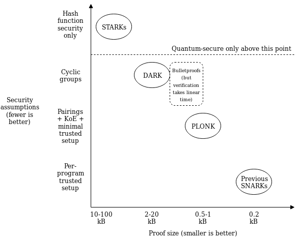
The second improvement is that the "fancy cryptography" it relies on is one single standardized component, called a "polynomial commitment". PLONK uses "Kate commitments", based on a trusted setup and elliptic curve pairings, but you can instead swap it out with other schemes, such as FRI (which would turn PLONK into a kind of STARK) or DARK (based on hidden-order groups). This means the scheme is theoretically compatible with any (achievable) tradeoff between proof size and security assumptions.
What this means is that use cases that require different tradeoffs between proof size and security assumptions (or developers that have different ideological positions about this question) can still share the bulk of the same tooling for "arithmetization" - the process for converting a program into a set of polynomial equations that the polynomial commitments are then used to check. If this kind of scheme becomes widely adopted, we can thus expect rapid progress in improving shared arithmetization techniques.
How PLONK works
Let us start with an explanation of how PLONK works, in a somewhat abstracted format that focuses on polynomial equations without immediately explaining how those equations are verified. A key ingredient in PLONK, as is the case in the QAPs used in SNARKs, is a procedure for converting a problem of the form "give me a value \(X\) such that a specific program \(P\) that I give you, when evaluated with \(X\) as an input, gives some specific result \(Y\)" into the problem "give me a set of values that satisfies a set of math equations". The program \(P\) can represent many things; for example the problem could be "give me a solution to this sudoku", which you would encode by setting \(P\) to be a sudoku verifier plus some initial values encoded and setting \(Y\) to \(1\) (ie. "yes, this solution is correct"), and a satisfying input \(X\) would be a valid solution to the sudoku. This is done by representing \(P\) as a circuit with logic gates for addition and multiplication, and converting it into a system of equations where the variables are the values on all the wires and there is one equation per gate (eg. \(x_6 = x_4 \cdot x_7\) for multiplication, \(x_8 = x_5 + x_9\) for addition).
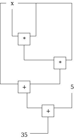
Here is an example of the problem of finding \(x\) such that \(P(x) = x^3 + x + 5 = 35\) (hint: \(x = 3\)):
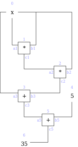
We can label the gates and wires as follows:
On the gates and wires, we have two types of constraints: gate constraints (equations between wires attached to the same gate, eg. \(a_1 \cdot b_1 = c_1\)) and copy constraints (claims about equality of different wires anywhere in the circuit, eg. \(a_0 = a_1 = b_1 = b_2 = a_3\) or \(c_0 = a_1\)). We will need to create a structured system of equations, which will ultimately reduce to a very small number of polynomial equations, to represent both.
In PLONK, the setup for these equations is as follows. Each equation is of the following form (think: \(L\) = left, \(R\) = right, \(O\) = output, \(M\) = multiplication, \(C\) = constant):
\[ \left(Q_{L_{i}}\right) a_{i}+\left(Q_{R_{i}}\right) b_{i}+\left(Q_{O_{i}}\right) c_{i}+\left(Q_{M_{i}}\right) a_{i} b_{i}+Q_{C_{i}}=0 \]
Each \(Q\) value is a constant; the constants in each equation (and the number of equations) will be different for each program. Each small-letter value is a variable, provided by the user: \(a_i\) is the left input wire of the \(i\)'th gate, \(b_i\) is the right input wire, and \(c_i\) is the output wire of the \(i\)'th gate. For an addition gate, we set:
\[ Q_{L_{i}}=1, Q_{R_{i}}=1, Q_{M_{i}}=0, Q_{O_{i}}=-1, Q_{C_{i}}=0 \]
Plugging these constants into the equation and simplifying gives us \(a_i + b_i - c_i = 0\), which is exactly the constraint that we want. For a multiplication gate, we set:
\[ Q_{L_{i}}=0, Q_{R_{i}}=0, Q_{M_{i}}=1, Q_{O_{i}}=-1, Q_{C_{i}}=0 \]
For a constant gate setting \(a_i\) to some constant \(x\), we set:
\[ Q_{L}=1, Q_{R}=0, Q_{M}=0, Q_{O}=0, Q_{C}=-x \]
You may have noticed that each end of a wire, as well as each wire in a set of wires that clearly must have the same value (eg. \(x\)), corresponds to a distinct variable; there's nothing so far forcing the output of one gate to be the same as the input of another gate (what we call "copy constraints"). PLONK does of course have a way of enforcing copy constraints, but we'll get to this later. So now we have a problem where a prover wants to prove that they have a bunch of \(x_{a_i}, x_{b_i}\) and \(x_{c_i}\) values that satisfy a bunch of equations that are of the same form. This is still a big problem, but unlike "find a satisfying input to this computer program" it's a very structured big problem, and we have mathematical tools to "compress" it.
From linear systems to polynomials
If you have read about STARKs or QAPs, the mechanism described in this next section will hopefully feel somewhat familiar, but if you have not that's okay too. The main ingredient here is to understand a polynomial as a mathematical tool for encapsulating a whole lot of values into a single object. Typically, we think of polynomials in "coefficient form", that is an expression like:
\[ y=x^{3}-5 x^{2}+7 x-2 \]
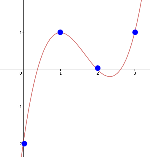
But we can also view polynomials in "evaluation form". For example, we can think of the above as being "the" degree \(< 4\) polynomial with evaluations \((-2, 1, 0, 1)\) at the coordinates \((0, 1, 2, 3)\) respectively.
Now here's the next step. Systems of many equations of the same form can be re-interpreted as a single equation over polynomials. For example, suppose that we have the system:
\[ \begin{array}{l}{2 x_{1}-x_{2}+3 x_{3}=8} \\ {x_{1}+4 x_{2}-5 x_{3}=5} \\ {8 x_{1}-x_{2}-x_{3}=-2}\end{array} \]
Let us define four polynomials in evaluation form: \(L(x)\) is the degree \(< 3\) polynomial that evaluates to \((2, 1, 8)\) at the coordinates \((0, 1, 2)\), and at those same coordinates \(M(x)\) evaluates to \((-1, 4, -1)\), \(R(x)\) to \((3, -5, -1)\) and \(O(x)\) to \((8, 5, -2)\) (it is okay to directly define polynomials in this way; you can use Lagrange interpolation to convert to coefficient form). Now, consider the equation:
\[ L(x) \cdot x_{1}+M(x) \cdot x_{2}+R(x) \cdot x_{3}-O(x)=Z(x) H(x) \]
Here, \(Z(x)\) is shorthand for \((x-0) \cdot (x-1) \cdot (x-2)\) - the minimal (nontrivial) polynomial that returns zero over the evaluation domain \((0, 1, 2)\). A solution to this equation (\(x_1 = 1, x_2 = 6, x_3 = 4, H(x) = 0\)) is also a solution to the original system of equations, except the original system does not need \(H(x)\). Notice also that in this case, \(H(x)\) is conveniently zero, but in more complex cases \(H\) may need to be nonzero.
So now we know that we can represent a large set of constraints within a small number of mathematical objects (the polynomials). But in the equations that we made above to represent the gate wire constraints, the \(x_1, x_2, x_3\) variables are different per equation. We can handle this by making the variables themselves polynomials rather than constants in the same way. And so we get:
\[ Q_{L}(x) a(x)+Q_{R}(x) b(x)+Q_{O}(x) c(x)+Q_{M}(x) a(x) b(x)+Q_{C}(x)=0 \]
As before, each \(Q\) polynomial is a parameter that can be generated from the program that is being verified, and the \(a\), \(b\), \(c\) polynomials are the user-provided inputs.
Copy constraints
Now, let us get back to "connecting" the wires. So far, all we have is a bunch of disjoint equations about disjoint values that are independently easy to satisfy: constant gates can be satisfied by setting the value to the constant and addition and multiplication gates can simply be satisfied by setting all wires to zero! To make the problem actually challenging (and actually represent the problem encoded in the original circuit), we need to add an equation that verifies "copy constraints": constraints such as \(a(5) = c(7)\), \(c(10) = c(12)\), etc. This requires some clever trickery.
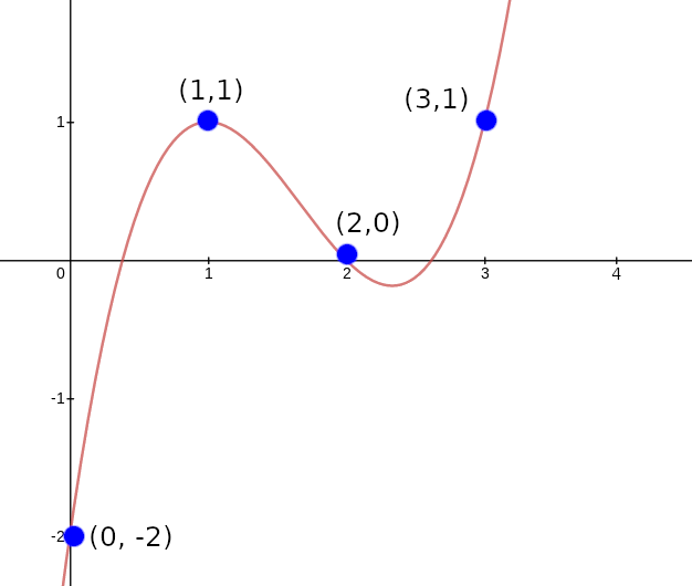
Our strategy will be to design a "coordinate pair accumulator", a polynomial \(p(x)\) which works as follows. First, let \(X(x)\) and \(Y(x)\) be two polynomials representing the \(x\) and \(y\) coordinates of a set of points (eg. to represent the set \(((0, -2), (1, 1), (2, 0), (3, 1))\) you might set \(X(x) = x\) and \(Y(x) = x^3 - 5x^2 + 7x - 2)\). Our goal will be to let \(p(x)\) represent all the points up to (but not including) the given position, so \(p(0)\) starts at \(1\), \(p(1)\) represents just the first point, \(p(2)\) the first and the second, etc. We will do this by "randomly" selecting two constants, \(v_1\) and \(v_2\), and constructing \(p(x)\) using the constraints \(p(0) = 1\) and \(p(x+1) = p(x) \cdot (v_1 + X(x) + v_2 \cdot Y(x))\) at least within the domain \((0, 1, 2, 3)\).
For example, letting \(v_1 = 3\) and \(v_2 = 2\), we get:
Notice that (aside from the first column) every \(p(x)\) value equals the value to the left of it multiplied by the value to the left and above it.
The result we care about is \(p(4) = -240\). Now, consider the case where instead of \(X(x) = x\), we set \(X(x) = \frac{2}{3} x^3 - 4x^2 + \frac{19}{3}x\) (that is, the polynomial that evaluates to \((0, 3, 2, 1)\) at the coordinates \((0, 1, 2, 3)\)). If you run the same procedure, you'll find that you also get \(p(4) = -240\). This is not a coincidence (in fact, if you randomly pick \(v_1\) and \(v_2\) from a sufficiently large field, it will almost never happen coincidentally). Rather, this happens because \(Y(1) = Y(3)\), so if you "swap the \(X\) coordinates" of the points \((1, 1)\) and \((3, 1)\) you're not changing the set of points, and because the accumulator encodes a set (as multiplication does not care about order) the value at the end will be the same.
Now we can start to see the basic technique that we will use to prove copy constraints. First, consider the simple case where we only want to prove copy constraints within one set of wires (eg. we want to prove \(a(1) = a(3)\)). We'll make two coordinate accumulators: one where \(X(x) = x\) and \(Y(x) = a(x)\), and the other where \(Y(x) = a(x)\) but \(X'(x)\) is the polynomial that evaluates to the permutation that flips (or otherwise rearranges) the values in each copy constraint; in the \(a(1) = a(3)\) case this would mean the permutation would start \(0 3 2 1 4...\). The first accumulator would be compressing \(((0, a(0)), (1, a(1)), (2, a(2)), (3, a(3)), (4, a(4))...\), the second \(((0, a(0)), (3, a(1)), (2, a(2)), (1, a(3)), (4, a(4))...\). The only way the two can give the same result is if \(a(1) = a(3)\).
To prove constraints between \(a\), \(b\) and \(c\), we use the same procedure, but instead "accumulate" together points from all three polynomials. We assign each of \(a\), \(b\), \(c\) a range of \(X\) coordinates (eg. \(a\) gets \(X_a(x) = x\) ie. \(0...n-1\), \(b\) gets \(X_b(x) = n+x\), ie. \(n...2n-1\), \(c\) gets \(X_c(x) = 2n+x\), ie. \(2n...3n-1\). To prove copy constraints that hop between different sets of wires, the "alternate" \(X\) coordinates would be slices of a permutation across all three sets. For example, if we want to prove \(a(2) = b(4)\) with \(n = 5\), then \(X'_a(x)\) would have evaluations \(\{0, 1, 9, 3, 4\}\) and \(X'_b(x)\) would have evaluations \(\{5, 6, 7, 8, 2\}\) (notice the \(2\) and \(9\) flipped, where \(9\) corresponds to the \(b_4\) wire). Often, \(X'_a(x)\), \(X'_b(x)\) and \(X'_c(x)\) are also called \(\sigma_a(x)\), \(\sigma_b(x)\) and \(\sigma_c(x)\).
We would then instead of checking equality within one run of the procedure (ie. checking \(p(4) = p'(4)\) as before), we would check the product of the three different runs on each side:
\[ p_{a}(n) \cdot p_{b}(n) \cdot p_{c}(n)=p_{a}^{\prime}(n) \cdot p_{b}^{\prime}(n) \cdot p_{c}^{\prime}(n) \]
The product of the three \(p(n)\) evaluations on each side accumulates all coordinate pairs in the \(a\), \(b\) and \(c\) runs on each side together, so this allows us to do the same check as before, except that we can now check copy constraints not just between positions within one of the three sets of wires \(a\), \(b\) or \(c\), but also between one set of wires and another (eg. as in \(a(2) = b(4)\)).
And that's all there is to it!
Putting it all together
In reality, all of this math is done not over integers, but over a prime field; check the section "A Modular Math Interlude" here for a description of what prime fields are. Also, for mathematical reasons perhaps best appreciated by reading and understanding this article on FFT implementation, instead of representing wire indices with \(x=0....n-1\), we'll use powers of \(\omega: 1, \omega, \omega ^2....\omega ^{n-1}\) where \(\omega\) is a high-order root-of-unity in the field. This changes nothing about the math, except that the coordinate pair accumulator constraint checking equation changes from \(p(x + 1) = p(x) \cdot (v_1 + X(x) + v_2 \cdot Y(x))\) to \(p(\omega \cdot x) = p(x) \cdot (v_1 + X(x) + v_2 \cdot Y(x))\), and instead of using \(0..n-1\), \(n..2n-1\), \(2n..3n-1\) as coordinates we use \(\omega^i, g \cdot \omega^i\) and \(g^2 \cdot \omega^i\) where \(g\) can be some random high-order element in the field.
Now let's write out all the equations we need to check. First, the main gate-constraint satisfaction check:
\[ Q_{L}(x) a(x)+Q_{R}(x) b(x)+Q_{O}(x) c(x)+Q_{M}(x) a(x) b(x)+Q_{C}(x)=0 \]
Then the polynomial accumulator transition constraint (note: think of "\(= Z(x) \cdot H(x)\)" as meaning "equals zero for all coordinates within some particular domain that we care about, but not necessarily outside of it"):
\[ \begin{array}{l}{P_{a}(\omega x)-P_{a}(x)\left(v_{1}+x+v_{2} a(x)\right) =Z(x) H_{1}(x)} \\ {P_{a^{\prime}}(\omega x)-P_{a^{\prime}}(x)\left(v_{1}+\sigma_{a}(x)+v_{2} a(x)\right)=Z(x) H_{2}(x)} \\ {P_{b}(\omega x)-P_{b}(x)\left(v_{1}+g x+v_{2} b(x)\right)=Z(x) H_{3}(x)} \\ {P_{b^{\prime}}(\omega x)-P_{b^{\prime}}(x)\left(v_{1}+\sigma_{b}(x)+v_{2} b(x)\right)=Z(x) H_{4}(x)} \\ {P_{c}(\omega x)-P_{c}(x)\left(v_{1}+g^{2} x+v_{2} c(x)\right)=Z(x) H_{5}(x)} \\ {P_{c^{\prime}}(\omega x)-P_{c^{\prime}}(x)\left(v_{1}+\sigma_{c}(x)+v_{2} c(x)\right)=Z(x) H_{6}(x)}\end{array} \]
Then the polynomial accumulator starting and ending constraints:
\[ \begin{array}{l}{P_{a}(1)=P_{b}(1)=P_{c}(1)=P_{a^{\prime}}(1)=P_{b^{\prime}}(1)=P_{c^{\prime}}(1)=1} \\ {P_{a}\left(\omega^{n}\right) P_{b}\left(\omega^{n}\right) P_{c}\left(\omega^{n}\right)=P_{a^{\prime}}\left(\omega^{n}\right) P_{b^{\prime}}\left(\omega^{n}\right) P_{c^{\prime}}\left(\omega^{n}\right)}\end{array} \]
The user-provided polynomials are:
The program-specific polynomials that the prover and verifier need to compute ahead of time are:
Note that the verifier need only store commitments to these polynomials. The only remaining polynomial in the above equations is \(Z(x) = (x - 1) \cdot (x - \omega) \cdot ... \cdot (x - \omega ^{n-1})\) which is designed to evaluate to zero at all those points. Fortunately, \(\omega\) can be chosen to make this polynomial very easy to evaluate: the usual technique is to choose \(\omega\) to satisfy \(\omega ^n = 1\), in which case \(Z(x) = x^n - 1\).
There is one nuance here: the constraint between \(P_a(\omega^{i+1})\) and \(P_a(\omega^i)\) can't be true across the entire circle of powers of \(\omega\); it's almost always false at \(\omega^{n-1}\) as the next coordinate is \(\omega^n = 1\) which brings us back to the start of the "accumulator"; to fix this, we can modify the constraint to say "either the constraint is true or \(x = \omega^{n-1}\)", which one can do by multiplying \(x - \omega^{n-1}\) into the constraint so it equals zero at that point.
The only constraint on \(v_1\) and \(v_2\) is that the user must not be able to choose \(a(x), b(x)\) or \(c(x)\) after \(v_1\) and \(v_2\) become known, so we can satisfy this by computing \(v_1\) and \(v_2\) from hashes of commitments to \(a(x), b(x)\) and \(c(x)\).
So now we've turned the program satisfaction problem into a simple problem of satisfying a few equations with polynomials, and there are some optimizations in PLONK that allow us to remove many of the polynomials in the above equations that I will not go into to preserve simplicity. But the polynomials themselves, both the program-specific parameters and the user inputs, are big. So the next question is, how do we get around this so we can make the proof short?
Polynomial commitments
A polynomial commitment is a short object that "represents" a polynomial, and allows you to verify evaluations of that polynomial, without needing to actually contain all of the data in the polynomial. That is, if someone gives you a commitment \(c\) representing \(P(x)\), they can give you a proof that can convince you, for some specific \(z\), what the value of \(P(z)\) is. There is a further mathematical result that says that, over a sufficiently big field, if certain kinds of equations (chosen before \(z\) is known) about polynomials evaluated at a random \(z\) are true, those same equations are true about the whole polynomial as well. For example, if \(P(z) \cdot Q(z) + R(z) = S(z) + 5\), then we know that it's overwhelmingly likely that \(P(x) \cdot Q(x) + R(x) = S(x) + 5\) in general. Using such polynomial commitments, we could very easily check all of the above polynomial equations above - make the commitments, use them as input to generate \(z\), prove what the evaluations are of each polynomial at \(z\), and then run the equations with these evaluations instead of the original polynomials. But how do these commitments work?
There are two parts: the commitment to the polynomial \(P(x) \rightarrow c\), and the opening to a value \(P(z)\) at some \(z\). To make a commitment, there are many techniques; one example is FRI, and another is Kate commitments which I will describe below. To prove an opening, it turns out that there is a simple generic "subtract-and-divide" trick: to prove that \(P(z) = a\), you prove that
\[ \frac{P(x)-a}{x-z} \]
is also a polynomial (using another polynomial commitment). This works because if the quotient is a polynomial (ie. it is not fractional), then \(x - z\) is a factor of \(P(x) - a\), so \((P(x) - a)(z) = 0\), so \(P(z) = a\). Try it with some polynomial, eg. \(P(x) = x^3 + 2 \cdot x^2 + 5\) with \((z = 6, a = 293)\), yourself; and try \((z = 6, a = 292)\) and see how it fails (if you're lazy, see WolframAlpha here vs here). Note also a generic optimization: to prove many openings of many polynomials at the same time, after committing to the outputs do the subtract-and-divide trick on a random linear combination of the polynomials and the outputs.
So how do the commitments themselves work? Kate commitments are, fortunately, much simpler than FRI. A trusted-setup procedure generates a set of elliptic curve points \(G, G \cdot s, G \cdot s^2\) .... \(G \cdot s^n\), as well as \(G_2 \cdot s\), where \(G\) and \(G_2\) are the generators of two elliptic curve groups and \(s\) is a secret that is forgotten once the procedure is finished (note that there is a multi-party version of this setup, which is secure as long as at least one of the participants forgets their share of the secret). These points are published and considered to be "the proving key" of the scheme; anyone who needs to make a polynomial commitment will need to use these points. A commitment to a degree-d polynomial is made by multiplying each of the first d+1 points in the proving key by the corresponding coefficient in the polynomial, and adding the results together.
Notice that this provides an "evaluation" of that polynomial at \(s\), without knowing \(s\). For example, \(x^3 + 2x^2+5\) would be represented by \((G \cdot s^3) + 2 \cdot (G \cdot s^2) + 5 \cdot G\). We can use the notation \([P]\) to refer to \(P\) encoded in this way (ie. \(G \cdot P(s)\)). When doing the subtract-and-divide trick, you can prove that the two polynomials actually satisfy the relation by using elliptic curve pairings: check that \(e([P] - G \cdot a, G_2) = e([Q], [x] - G_2 \cdot z)\) as a proxy for checking that \(P(x) - a = Q(x) \cdot (x - z)\).
But there are more recently other types of polynomial commitments coming out too. A new scheme called DARK ("Diophantine arguments of knowledge") uses "hidden order groups" such as class groups to implement another kind of polynomial commitment. Hidden order groups are unique because they allow you to compress arbitrarily large numbers into group elements, even numbers much larger than the size of the group element, in a way that can't be "spoofed"; constructions from VDFs to accumulators to range proofs to polynomial commitments can be built on top of this. Another option is to use bulletproofs, using regular elliptic curve groups at the cost of the proof taking much longer to verify. Because polynomial commitments are much simpler than full-on zero knowledge proof schemes, we can expect more such schemes to get created in the future.
Recap
To finish off, let's go over the scheme again. Given a program \(P\), you convert it into a circuit, and generate a set of equations that look like this:
\[ \left(Q_{L_{i}}\right) a_{i}+\left(Q_{R_{i}}\right) b_{i}+\left(Q_{O_{i}}\right) c_{i}+\left(Q_{M_{i}}\right) a_{i} b_{i}+Q_{C_{i}}=0 \]
You then convert this set of equations into a single polynomial equation:
\[ Q_{L}(x) a(x)+Q_{R}(x) b(x)+Q_{O}(x) c(x)+Q_{M}(x) a(x) b(x)+Q_{C}(x)=0 \]
You also generate from the circuit a list of copy constraints. From these copy constraints you generate the three polynomials representing the permuted wire indices: \(\sigma_a(x), \sigma_b(x), \sigma_c(x)\). To generate a proof, you compute the values of all the wires and convert them into three polynomials: \(a(x), b(x), c(x)\). You also compute six "coordinate pair accumulator" polynomials as part of the permutation-check argument. Finally you compute the cofactors \(H_i(x)\).
There is a set of equations between the polynomials that need to be checked; you can do this by making commitments to the polynomials, opening them at some random \(z\) (along with proofs that the openings are correct), and running the equations on these evaluations instead of the original polynomials. The proof itself is just a few commitments and openings and can be checked with a few equations. And that's all there is to it!