STARKs, Part I: Proofs with Polynomials
2017 Nov 09
See all posts
STARKs, Part I: Proofs with Polynomials
Special thanks to Eli Ben-Sasson for ongoing help, explanations
and review, coming up with some of the examples used in this post, and
most crucially of all inventing a lot of this stuff; thanks to Hsiao-wei
Wang for reviewing
Hopefully many people by now have heard of ZK-SNARKs,
the general-purpose succinct zero knowledge proof technology that can be
used for all sorts of usecases ranging from verifiable computation to
privacy-preserving cryptocurrency. What you might not know is that
ZK-SNARKs have a newer, shinier cousin: ZK-STARKs. With the T standing
for "transparent", ZK-STARKs resolve one of the primary weaknesses of
ZK-SNARKs, its reliance on a "trusted setup". They also come with much
simpler cryptographic assumptions, avoiding the need for elliptic
curves, pairings and the knowledge-of-exponent assumption and instead
relying purely on hashes and information theory; this also means that
they are secure even against attackers with quantum computers.
However, this comes at a cost: the size of a proof goes up from 288
bytes to a few hundred kilobytes. Sometimes the cost will not be worth
it, but at other times, particularly in the context of public blockchain
applications where the need for trust minimization is high, it may well
be. And if elliptic curves break or quantum computers do come
around, it definitely will be.
So how does this other kind of zero knowledge proof work? First of
all, let us review what a general-purpose succinct ZKP does. Suppose
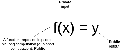
that you have a (public) function \(f\), a (private) input \(x\) and a (public) output \(y\). You want to prove that you know an
\(x\) such that \(f(x) = y\), without revealing what \(x\) is. Furthermore, for the proof to be
succinct, you want it to be verifiable much more quickly than
computing \(f\) itself.
Let's go through a few examples:
- \(f\) is a computation that takes
two weeks to run on a regular computer, but two hours on a data center.
You send the data center the computation (ie. the code to run \(f\) ), the data center runs it, and gives
back the answer \(y\) with a proof. You
verify the proof in a few milliseconds, and are convinced that \(y\) actually is the answer.
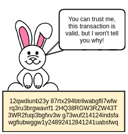
- You have an encrypted transaction, of the form "\(X_1\) was my old balance. \(X_2\) was your old balance. \(X_3\) is my new balance. \(X_4\) is your new balance". You want to
create a proof that this transaction is valid (specifically, old and new
balances are non-negative, and the decrease in my balance cancels out
the increase in your balance). \(x\)
can be the pair of encryption keys, and \(f\) can be a function which contains as a
built-in public input the transaction, takes as input the keys, decrypts
the transaction, performs the check, and returns 1 if it passes and 0 if
it does not. \(y\) would of course be
1.
- You have a blockchain like Ethereum, and you download the most
recent block. You want a proof that this block is valid, and that this
block is at the tip of a chain where every block in the chain is valid.
You ask an existing full node to provide such a proof. \(x\) is the entire blockchain (yes, all ??
gigabytes of it), \(f\) is a function
that processes it block by block, verifies the validity and outputs the
hash of the last block, and \(y\) is
the hash of the block you just downloaded.
So what's so hard about all this? As it turns out, the zero
knowledge (ie. privacy) guarantee is (relatively!) easy to provide;
there are a bunch of ways to convert any computation into an instance of
something like the three color graph problem, where a three-coloring of
the graph corresponds to a solution of the original problem, and then
use a traditional zero knowledge proof protocol to prove that you have a
valid graph coloring without revealing what it is. This excellent
post by Matthew Green from 2014 describes this in some detail.
The much harder thing to provide is succinctness.
Intuitively speaking, proving things about computation succinctly is
hard because computation is incredibly fragile. If you have a
long and complex computation, and you as an evil genie have the ability
to flip a 0 to a 1 anywhere in the middle of the computation, then in
many cases even one flipped bit will be enough to make the computation
give a completely different result. Hence, it's hard to see how you can
do something like randomly sampling a computation trace in order to
gauge its correctness, as it's just too easy to miss that "one evil
bit". However, with some fancy math, it turns out that you can.
The general very high level intuition is that the protocols that
accomplish this use similar math to what is used in erasure coding,
which is frequently used to make data fault-tolerant. If you
have a piece of data, and you encode the data as a line, then you can
pick out four points on the line. Any two of those four points are
enough to reconstruct the original line, and therefore also give you the
other two points. Furthermore, if you make even the slightest change to
the data, then it is guaranteed at least three of those four points. You
can also encode the data as a degree-1,000,000 polynomial, and pick out
2,000,000 points on the polynomial; any 1,000,001 of those points will
recover the original data and therefore the other points, and any
deviation in the original data will change at least 1,000,000 points.
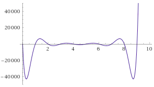
The algorithms shown here will make heavy use of polynomials in this way
for error amplification.
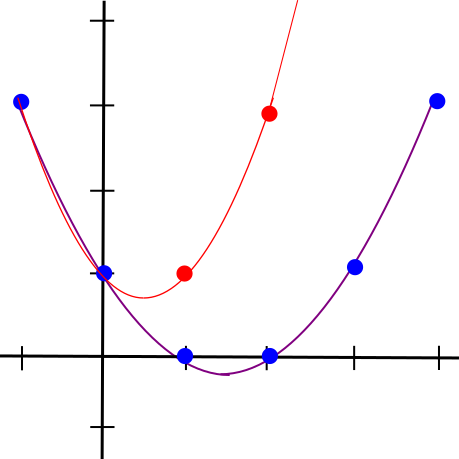
Changing even one point in the original data will lead to large
changes in a polynomial's trajectory
A Somewhat Simple Example
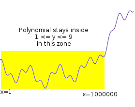
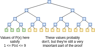
Suppose that you want to prove that you have a polynomial \(P\) such that \(P(x)\) is an integer with \(0 \leq P(x) \leq 9\) for all \(x\) from 1 to 1 million. This is a simple
instance of the fairly common task of "range checking"; you might
imagine this kind of check being used to verify, for example, that a set
of account balances is still positive after applying some set of
transactions. If it were \(1 \leq P(x) \leq
9\), this could be part of checking that the values form a
correct Sudoku solution.
The "traditional" way to prove this would be to just show all
1,000,000 points, and verify it by checking the values. However, we want
to see if we can make a proof that can be verified in less than
1,000,000 steps. Simply randomly checking evaluations of \(P\) won't do; there's always the
possibility that a malicious prover came up with a \(P\) which satisfies the constraint in
999,999 places but does not satisfy it in the last one, and random
sampling only a few values will almost always miss that value. So what
can we do?
Let's mathematically transform the problem somewhat. Let \(C(x)\) be a constraint checking
polynomial; \(C(x) = 0\) if \(0 \leq x \leq 9\) and is nonzero otherwise.
There's a simple way to construct \(C(x)\): \(x \cdot
(x-1) \cdot (x-2) \cdot \ldots(x-9)\) (we'll assume all of our
polynomials and other values use exclusively integers, so we don't need
to worry about numbers in between).
Now, the problem becomes: prove that you know \(P\) such that \(C(P(x)) = 0\) for all \(x\) from 1 to 1,000,000. Let \(Z(x) = (x-1) \cdot (x-2) \cdot \ldots
(x-1000000)\). It's a known mathematical fact that any
polynomial which equals zero at all \(x\) from 1 to 1,000,000 is a multiple of
\(Z(x)\). Hence, the problem can now be
transformed again: prove that you know \(P\) and \(D\) such that \(C(P(x)) = Z(x) \cdot D(x)\) for all \(x\) (note that if you know a suitable \(C(P(x))\) then dividing it by \(Z(x)\) to compute \(D(x)\) is not too difficult; you can use long polynomial
division or more realistically a faster algorithm based on FFTs).
Now, we've converted our original statement into something that looks
mathematically clean and possibly quite provable.
So how does one prove this claim? We can imagine the proof process as
a three-step communication between a prover and a verifier: the prover
sends some information, then the verifier sends some requests, then the
prover sends some more information. First, the prover commits to (ie.
makes a Merkle tree and sends the verifier the root hash of) the
evaluations of \(P(x)\) and \(D(x)\) for all \(x\) from 1 to 1 billion (yes, billion).
This includes the 1 million points where \(0
\leq P(x) \leq 9\) as well as the 999 million points where that
(probably) is not the case.
We assume the verifier already knows the evaluation of \(Z(x)\) at all of these points; the \(Z(x)\) is like a "public verification key"
for this scheme that everyone must know ahead of time (clients that do
not have the space to store \(Z(x)\) in
its entirety can simply store the Merkle root of \(Z(x)\) and require the prover to also
provide branches for every \(Z(x)\)
value that the verifier needs to query; alternatively, there are some
number fields over which \(Z(x)\) for
certain \(x\) is very easy to
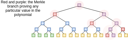
calculate). After receiving the commitment (ie. Merkle root) the
verifier then selects a random 16 \(x\)
values between 1 and 1 billion, and asks the prover to provide the
Merkle branches for \(P(x)\) and \(D(x)\) there. The prover provides these
values, and the verifier checks that (i) the branches match the Merkle
root that was provided earlier, and (ii) \(C(P(x))\) actually equals \(Z(x) \cdot D(x)\) in all 16 cases.
We know that this proof perfect completeness - if you
actually know a suitable \(P(x)\), then
if you calculate \(D(x)\) and construct
the proof correctly it will always pass all 16 checks. But what about
soundness - that is, if a malicious prover provides a bad \(P(x)\), what is the minimum probability
that they will get caught? We can analyze as follows. Because \(C(P(x))\) is a degree-10 polynomial
composed with a degree-1,000,000 polynomial, its degree will be at most
10,000,000. In general, we know that two different degree-\(N\) polynomials agree on at most \(N\) points; hence, a degree-10,000,000
polynomial which is not equal to any polynomial which always equals
\(Z(x) \cdot D(x)\) for some \(x\) will necessarily disagree with them all
at at least 990,000,000 points. Hence, the probability that a bad \(P(x)\) will get caught in even one round is
already 99%; with 16 checks, the probability of getting caught goes up
to \(1 - 10^{-32}\); that is to say,
the scheme is about as hard to spoof as it is to compute a hash
collision.
So... what did we just do? We used polynomials to "boost" the error in
any bad solution, so that any incorrect solution to the original
problem, which would have required a million checks to find directly,
turns into a solution to the verification protocol that can get flagged
as erroneous at 99% of the time with even a single check.
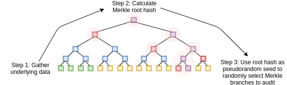
We can convert this three-step mechanism into a non-interactive
proof, which can be broadcasted by a single prover once and then
verified by anyone, using the Fiat-Shamir
heuristic. The prover first builds up a Merkle tree of the \(P(x)\) and \(D(x)\) values, and computes the root hash
of the tree. The root itself is then used as the source of entropy that
determines what branches of the tree the prover needs to provide. The
prover then broadcasts the Merkle root and the branches together as the
proof. The computation is all done on the prover side; the process of
computing the Merkle root from the data, and then using that to select
the branches that get audited, effectively substitutes the need for an
interactive verifier.
The only thing a malicious prover without a valid \(P(x)\) can do is try to make a valid proof
over and over again until eventually they get extremely lucky
with the branches that a Merkle root that they compute selects, but with
a soundness of \(1 - 10^{-32}\) (ie.
probability of at least \(1 -
10^{-32}\) that a given attempted fake proof will fail the check)
it would take a malicious prover billions of years to make a passable
proof.
Going Further
To illustrate the power of this technique, let's use it to do
something a little less trivial: prove that you know the millionth
Fibonacci number. To accomplish this, we'll prove that you have
knowledge of a polynomial which represents a computation tape, with
\(P(x)\) representing the \(x\)th Fibonacci number. The constraint
checking polynomial will now hop across three x-coordinates: \(C(x_1, x_2, x_3) = x_3-x_2-x_1\) (notice
how if \(C(P(x), P(x+1), P(x+2)) = 0\)
for all \(x\) then \(P(x)\) represents a Fibonacci
sequence).
The translated problem becomes: prove that you know \(P\) and \(D\) such that \(C(P(x), P(x+1), P(x+2)) = Z(x) \cdot
D(x)\). For each of the 16 indices that the proof audits, the
prover will need to provide Merkle branches for \(P(x)\), \(P(x+1)\), \(P(x+2)\) and \(D(x)\). The prover will additionally need
to provide Merkle branches to show that \(P(0)
= P(1) = 1\). Otherwise, the entire process is the same.
Now, to accomplish this in reality there are two problems that need
to be resolved. The first problem is that if we actually try to work
with regular numbers the solution would not be efficient in
practice, because the numbers themselves very easily get extremely
large. The millionth Fibonacci number, for example, has 208988 digits.
If we actually want to achieve succinctness in practice, instead of
doing these polynomials with regular numbers, we need to use finite
fields - number systems that still follow the same arithmetic laws we
know and love, like \(a \cdot (b+c) = (a\cdot
b) + (a\cdot c)\) and \((a^2 - b^2) =
(a-b) \cdot (a+b)\), but where each number is guaranteed to take
up a constant amount of space. Proving claims about the millionth
Fibonacci number would then require a more complicated design that
implements big-number arithmetic on top of this finite field
math.
The simplest possible finite field is modular arithmetic; that is,
replace every instance of \(a + b\)
with \(a + b \mod{N}\) for some prime
\(N\), do the same for subtraction and
multiplication, and for division use modular
inverses (eg. if \(N = 7\), then
\(3 + 4 = 0\), \(2 + 6 = 1\), \(3
\cdot 4 = 5\), \(4 / 2 = 2\) and
\(5 / 2 = 6\)). You can learn more
about these kinds of number systems from my description on prime fields
here
(search "prime field" in the page) or this Wikipedia
article on modular arithmetic (the articles that you'll find by
searching directly for "finite fields" and "prime fields" unfortunately
tend to be very complicated and go straight into abstract algebra, don't
bother with those).
Second, you might have noticed that in my above proof sketch for
soundness I neglected to cover one kind of attack: what if, instead of a
plausible degree-1,000,000 \(P(x)\) and
degree-9,000,000 \(D(x)\), the attacker
commits to some values that are not on any such
relatively-low-degree polynomial? Then, the argument that an invalid
\(C(P(x))\) must differ from any valid
\(C(P(x))\) on at least 990 million
points does not apply, and so different and much more effective kinds of
attacks are possible. For example, an attacker could generate a
random value \(p\) for every \(x\), then compute \(d = C(p) / Z(x)\) and commit to these
values in place of \(P(x)\) and \(D(x)\). These values would not be on any
kind of low-degree polynomial, but they would pass the
test.
It turns out that this possibility can be effectively defended
against, though the tools for doing so are fairly complex, and so you
can quite legitimately say that they make up the bulk of the
mathematical innovation in STARKs. Also, the solution has a limitation:
you can weed out commitments to data that are very far from any
degree-1,000,000 polynomial (eg. you would need to change 20% of all the
values to make it a degree-1,000,000 polynomial), but you cannot weed
out commitments to data that only differ from a polynomial in only one
or two coordinates. Hence, what these tools will provide is proof of
proximity - proof that most of the points on \(P\) and \(D\) correspond to the right kind of
polynomial.
As it turns out, this is sufficient to make a proof, though there are
two "catches". First, the verifier needs to check a few more indices to
make up for the additional room for error that this limitation
introduces. Second, if we are doing "boundary constraint checking" (eg.
verifying \(P(0) = P(1) = 1\) in the
Fibonacci example above), then we need to extend the proof of proximity
to not only prove that most points are on the same polynomial, but also
prove that those two specific points (or whatever other number
of specific points you want to check) are on that polynomial.
In the next part of this series, I will describe the solution to
proximity checking in much more detail, and in the third part I will
describe how more complex constraint functions can be constructed to
check not just Fibonacci numbers and ranges, but also arbitrary
computation.
STARKs, Part I: Proofs with Polynomials
2017 Nov 09 See all postsSpecial thanks to Eli Ben-Sasson for ongoing help, explanations and review, coming up with some of the examples used in this post, and most crucially of all inventing a lot of this stuff; thanks to Hsiao-wei Wang for reviewing
Hopefully many people by now have heard of ZK-SNARKs, the general-purpose succinct zero knowledge proof technology that can be used for all sorts of usecases ranging from verifiable computation to privacy-preserving cryptocurrency. What you might not know is that ZK-SNARKs have a newer, shinier cousin: ZK-STARKs. With the T standing for "transparent", ZK-STARKs resolve one of the primary weaknesses of ZK-SNARKs, its reliance on a "trusted setup". They also come with much simpler cryptographic assumptions, avoiding the need for elliptic curves, pairings and the knowledge-of-exponent assumption and instead relying purely on hashes and information theory; this also means that they are secure even against attackers with quantum computers.
However, this comes at a cost: the size of a proof goes up from 288 bytes to a few hundred kilobytes. Sometimes the cost will not be worth it, but at other times, particularly in the context of public blockchain applications where the need for trust minimization is high, it may well be. And if elliptic curves break or quantum computers do come around, it definitely will be.
So how does this other kind of zero knowledge proof work? First of all, let us review what a general-purpose succinct ZKP does. Suppose that you have a (public) function \(f\), a (private) input \(x\) and a (public) output \(y\). You want to prove that you know an \(x\) such that \(f(x) = y\), without revealing what \(x\) is. Furthermore, for the proof to be succinct, you want it to be verifiable much more quickly than computing \(f\) itself.
Let's go through a few examples:
So what's so hard about all this? As it turns out, the zero knowledge (ie. privacy) guarantee is (relatively!) easy to provide; there are a bunch of ways to convert any computation into an instance of something like the three color graph problem, where a three-coloring of the graph corresponds to a solution of the original problem, and then use a traditional zero knowledge proof protocol to prove that you have a valid graph coloring without revealing what it is. This excellent post by Matthew Green from 2014 describes this in some detail.
The much harder thing to provide is succinctness. Intuitively speaking, proving things about computation succinctly is hard because computation is incredibly fragile. If you have a long and complex computation, and you as an evil genie have the ability to flip a 0 to a 1 anywhere in the middle of the computation, then in many cases even one flipped bit will be enough to make the computation give a completely different result. Hence, it's hard to see how you can do something like randomly sampling a computation trace in order to gauge its correctness, as it's just too easy to miss that "one evil bit". However, with some fancy math, it turns out that you can.
The general very high level intuition is that the protocols that accomplish this use similar math to what is used in erasure coding, which is frequently used to make data fault-tolerant. If you have a piece of data, and you encode the data as a line, then you can pick out four points on the line. Any two of those four points are enough to reconstruct the original line, and therefore also give you the other two points. Furthermore, if you make even the slightest change to the data, then it is guaranteed at least three of those four points. You can also encode the data as a degree-1,000,000 polynomial, and pick out 2,000,000 points on the polynomial; any 1,000,001 of those points will recover the original data and therefore the other points, and any deviation in the original data will change at least 1,000,000 points. The algorithms shown here will make heavy use of polynomials in this way for error amplification.
Changing even one point in the original data will lead to large changes in a polynomial's trajectory
A Somewhat Simple Example
Suppose that you want to prove that you have a polynomial \(P\) such that \(P(x)\) is an integer with \(0 \leq P(x) \leq 9\) for all \(x\) from 1 to 1 million. This is a simple instance of the fairly common task of "range checking"; you might imagine this kind of check being used to verify, for example, that a set of account balances is still positive after applying some set of transactions. If it were \(1 \leq P(x) \leq 9\), this could be part of checking that the values form a correct Sudoku solution.
The "traditional" way to prove this would be to just show all 1,000,000 points, and verify it by checking the values. However, we want to see if we can make a proof that can be verified in less than 1,000,000 steps. Simply randomly checking evaluations of \(P\) won't do; there's always the possibility that a malicious prover came up with a \(P\) which satisfies the constraint in 999,999 places but does not satisfy it in the last one, and random sampling only a few values will almost always miss that value. So what can we do?
Let's mathematically transform the problem somewhat. Let \(C(x)\) be a constraint checking polynomial; \(C(x) = 0\) if \(0 \leq x \leq 9\) and is nonzero otherwise. There's a simple way to construct \(C(x)\): \(x \cdot (x-1) \cdot (x-2) \cdot \ldots(x-9)\) (we'll assume all of our polynomials and other values use exclusively integers, so we don't need to worry about numbers in between).
Now, the problem becomes: prove that you know \(P\) such that \(C(P(x)) = 0\) for all \(x\) from 1 to 1,000,000. Let \(Z(x) = (x-1) \cdot (x-2) \cdot \ldots (x-1000000)\). It's a known mathematical fact that any polynomial which equals zero at all \(x\) from 1 to 1,000,000 is a multiple of \(Z(x)\). Hence, the problem can now be transformed again: prove that you know \(P\) and \(D\) such that \(C(P(x)) = Z(x) \cdot D(x)\) for all \(x\) (note that if you know a suitable \(C(P(x))\) then dividing it by \(Z(x)\) to compute \(D(x)\) is not too difficult; you can use long polynomial division or more realistically a faster algorithm based on FFTs). Now, we've converted our original statement into something that looks mathematically clean and possibly quite provable.
So how does one prove this claim? We can imagine the proof process as a three-step communication between a prover and a verifier: the prover sends some information, then the verifier sends some requests, then the prover sends some more information. First, the prover commits to (ie. makes a Merkle tree and sends the verifier the root hash of) the evaluations of \(P(x)\) and \(D(x)\) for all \(x\) from 1 to 1 billion (yes, billion). This includes the 1 million points where \(0 \leq P(x) \leq 9\) as well as the 999 million points where that (probably) is not the case.
We assume the verifier already knows the evaluation of \(Z(x)\) at all of these points; the \(Z(x)\) is like a "public verification key" for this scheme that everyone must know ahead of time (clients that do not have the space to store \(Z(x)\) in its entirety can simply store the Merkle root of \(Z(x)\) and require the prover to also provide branches for every \(Z(x)\) value that the verifier needs to query; alternatively, there are some number fields over which \(Z(x)\) for certain \(x\) is very easy to calculate). After receiving the commitment (ie. Merkle root) the verifier then selects a random 16 \(x\) values between 1 and 1 billion, and asks the prover to provide the Merkle branches for \(P(x)\) and \(D(x)\) there. The prover provides these values, and the verifier checks that (i) the branches match the Merkle root that was provided earlier, and (ii) \(C(P(x))\) actually equals \(Z(x) \cdot D(x)\) in all 16 cases.
We know that this proof perfect completeness - if you actually know a suitable \(P(x)\), then if you calculate \(D(x)\) and construct the proof correctly it will always pass all 16 checks. But what about soundness - that is, if a malicious prover provides a bad \(P(x)\), what is the minimum probability that they will get caught? We can analyze as follows. Because \(C(P(x))\) is a degree-10 polynomial composed with a degree-1,000,000 polynomial, its degree will be at most 10,000,000. In general, we know that two different degree-\(N\) polynomials agree on at most \(N\) points; hence, a degree-10,000,000 polynomial which is not equal to any polynomial which always equals \(Z(x) \cdot D(x)\) for some \(x\) will necessarily disagree with them all at at least 990,000,000 points. Hence, the probability that a bad \(P(x)\) will get caught in even one round is already 99%; with 16 checks, the probability of getting caught goes up to \(1 - 10^{-32}\); that is to say, the scheme is about as hard to spoof as it is to compute a hash collision.
So... what did we just do? We used polynomials to "boost" the error in any bad solution, so that any incorrect solution to the original problem, which would have required a million checks to find directly, turns into a solution to the verification protocol that can get flagged as erroneous at 99% of the time with even a single check.
We can convert this three-step mechanism into a non-interactive proof, which can be broadcasted by a single prover once and then verified by anyone, using the Fiat-Shamir heuristic. The prover first builds up a Merkle tree of the \(P(x)\) and \(D(x)\) values, and computes the root hash of the tree. The root itself is then used as the source of entropy that determines what branches of the tree the prover needs to provide. The prover then broadcasts the Merkle root and the branches together as the proof. The computation is all done on the prover side; the process of computing the Merkle root from the data, and then using that to select the branches that get audited, effectively substitutes the need for an interactive verifier.
The only thing a malicious prover without a valid \(P(x)\) can do is try to make a valid proof over and over again until eventually they get extremely lucky with the branches that a Merkle root that they compute selects, but with a soundness of \(1 - 10^{-32}\) (ie. probability of at least \(1 - 10^{-32}\) that a given attempted fake proof will fail the check) it would take a malicious prover billions of years to make a passable proof.
Going Further
To illustrate the power of this technique, let's use it to do something a little less trivial: prove that you know the millionth Fibonacci number. To accomplish this, we'll prove that you have knowledge of a polynomial which represents a computation tape, with \(P(x)\) representing the \(x\)th Fibonacci number. The constraint checking polynomial will now hop across three x-coordinates: \(C(x_1, x_2, x_3) = x_3-x_2-x_1\) (notice how if \(C(P(x), P(x+1), P(x+2)) = 0\) for all \(x\) then \(P(x)\) represents a Fibonacci sequence).
The translated problem becomes: prove that you know \(P\) and \(D\) such that \(C(P(x), P(x+1), P(x+2)) = Z(x) \cdot D(x)\). For each of the 16 indices that the proof audits, the prover will need to provide Merkle branches for \(P(x)\), \(P(x+1)\), \(P(x+2)\) and \(D(x)\). The prover will additionally need to provide Merkle branches to show that \(P(0) = P(1) = 1\). Otherwise, the entire process is the same.
Now, to accomplish this in reality there are two problems that need to be resolved. The first problem is that if we actually try to work with regular numbers the solution would not be efficient in practice, because the numbers themselves very easily get extremely large. The millionth Fibonacci number, for example, has 208988 digits. If we actually want to achieve succinctness in practice, instead of doing these polynomials with regular numbers, we need to use finite fields - number systems that still follow the same arithmetic laws we know and love, like \(a \cdot (b+c) = (a\cdot b) + (a\cdot c)\) and \((a^2 - b^2) = (a-b) \cdot (a+b)\), but where each number is guaranteed to take up a constant amount of space. Proving claims about the millionth Fibonacci number would then require a more complicated design that implements big-number arithmetic on top of this finite field math.
The simplest possible finite field is modular arithmetic; that is, replace every instance of \(a + b\) with \(a + b \mod{N}\) for some prime \(N\), do the same for subtraction and multiplication, and for division use modular inverses (eg. if \(N = 7\), then \(3 + 4 = 0\), \(2 + 6 = 1\), \(3 \cdot 4 = 5\), \(4 / 2 = 2\) and \(5 / 2 = 6\)). You can learn more about these kinds of number systems from my description on prime fields here (search "prime field" in the page) or this Wikipedia article on modular arithmetic (the articles that you'll find by searching directly for "finite fields" and "prime fields" unfortunately tend to be very complicated and go straight into abstract algebra, don't bother with those).
Second, you might have noticed that in my above proof sketch for soundness I neglected to cover one kind of attack: what if, instead of a plausible degree-1,000,000 \(P(x)\) and degree-9,000,000 \(D(x)\), the attacker commits to some values that are not on any such relatively-low-degree polynomial? Then, the argument that an invalid \(C(P(x))\) must differ from any valid \(C(P(x))\) on at least 990 million points does not apply, and so different and much more effective kinds of attacks are possible. For example, an attacker could generate a random value \(p\) for every \(x\), then compute \(d = C(p) / Z(x)\) and commit to these values in place of \(P(x)\) and \(D(x)\). These values would not be on any kind of low-degree polynomial, but they would pass the test.
It turns out that this possibility can be effectively defended against, though the tools for doing so are fairly complex, and so you can quite legitimately say that they make up the bulk of the mathematical innovation in STARKs. Also, the solution has a limitation: you can weed out commitments to data that are very far from any degree-1,000,000 polynomial (eg. you would need to change 20% of all the values to make it a degree-1,000,000 polynomial), but you cannot weed out commitments to data that only differ from a polynomial in only one or two coordinates. Hence, what these tools will provide is proof of proximity - proof that most of the points on \(P\) and \(D\) correspond to the right kind of polynomial.
As it turns out, this is sufficient to make a proof, though there are two "catches". First, the verifier needs to check a few more indices to make up for the additional room for error that this limitation introduces. Second, if we are doing "boundary constraint checking" (eg. verifying \(P(0) = P(1) = 1\) in the Fibonacci example above), then we need to extend the proof of proximity to not only prove that most points are on the same polynomial, but also prove that those two specific points (or whatever other number of specific points you want to check) are on that polynomial.
In the next part of this series, I will describe the solution to proximity checking in much more detail, and in the third part I will describe how more complex constraint functions can be constructed to check not just Fibonacci numbers and ranges, but also arbitrary computation.